Free Genetics tool
 Free Genetics tool
Hardy-Weinberg Equilibrium Calculator
The Hardy-Weinberg Equilibrium Calculator determines expected genotype frequencies ($p^2 + 2pq + q^2 = 1$) from observed allele counts and evaluates equilibrium via chi-square testing. Hardy-Weinberg equilibrium is the null model of population genetics: if allele frequencies hold, genotype counts should sit at p², 2pq and q². This calculator derives p and q from your counts, prints the expected numbers, runs the chi-square test against them, and tells you whether the deviation is big enough to matter.
Hardy-Weinberg Equilibrium Calculator: result
| Genotype | Observed | Expected | (O − E)² ÷ E |
|---|---|---|---|
| AA | 48 | 40.96 | 1.21 |
| Aa | 32 | 46.08 | 4.302 |
| aa | 20 | 12.96 | 3.824 |
At a glance
- What it does: Derives p and q from your genotype counts, prints expected numbers, and runs a chi-square test at the 5% level.
- Who it is for: For students and researchers checking whether a sample is consistent with random mating at one locus.
- Typical result: Reports chi-square, per-genotype contributions, and a plain statement of what the comparison shows.
How to use the hardy-weinberg equilibrium calculator
- Keep counts mode if you have genotype tallies; switch to frequency mode if you only know p (for example from a published study) and want the expected distribution. prefill →
- Enter the observed AA, Aa and aa counts. p is estimated from them as (2AA + Aa) ÷ 2N rather than entered by hand. prefill →
- Read the expected AA / Aa / aa line: those are the counts Hardy-Weinberg predicts for your sample size.
- Check the chi-square value against 3.84: above it, the deviation is significant at the standard 5% level; below it, the sample is consistent with equilibrium.
- Use the chi-square components table to see which genotype is driving a significant result: the largest (O − E)² ÷ E term is the culprit.
Hardy-Weinberg Equilibrium: the formula & its source
Allele frequencies are estimated from the same sample (each AA contributes two dominant alleles, each Aa one of each):
p̂ = (2NAA + NAa) ÷ 2N · EAA = p²N · EAa = 2pqN · Eaa = q²N
The goodness-of-fit statistic sums each squared deviation weighted by its expected value, with one degree of freedom because p was estimated from the data:
χ² = Σ (O − E)² ÷ E → critical value 3.84 (α = 0.05, df = 1)
Above 3.84 the observed counts are unlikely to come from a population in equilibrium; at or below it, sampling noise explains the difference.
For genetic loci governed by three alleles (e.g. human ABO blood groups or tri-allelic microsatellites), calculate genotype frequencies and Chi-square tests with our 3-allele Hardy-Weinberg calculator.
| Symbol | Meaning | Unit | Typical range |
|---|---|---|---|
p | dominant allele frequency estimated from the counts | proportion | 0 to 1 |
q | recessive allele frequency, one minus p | proportion | 0 to 1 |
E | expected count for each genotype under equilibrium | individuals | 0 to sample size |
chi | chi-square statistic summed across the three genotypes | units | 0 upward; 3.84 is the 5% cut-off |
Hardy-Weinberg Equilibrium: worked example
Worked example: the defaults (48 AA, 32 Aa, 20 aa). N = 100, p = (2 × 48 + 32) ÷ 200 = 0.64, q = 0.36. Expected counts are 40.96 AA, 46.08 Aa and 12.96 aa. χ² = (48 − 40.96)²/40.96 + (32 − 46.08)²/46.08 + (20 − 12.96)²/12.96 = 9.34, well above 3.84. The equilibrium is ruled out. The signal is the heterozygote deficit: 32 observed against 46.08 expected, exactly the pattern inbreeding or population subdivision produces.
Example B: frequency mode, no test
Example B: frequency mode. Switch Input to Allele frequency only, keep p at 0.64 and the sample at 100. The page prints expected counts of 40.96 AA, 46.08 Aa and 12.96 aa and skips the test, because there is nothing observed to compare against. This view suits planning a screen or checking a sample against a published frequency, and it is also the quickest way to see how sensitive the carrier count is to a small shift in p.
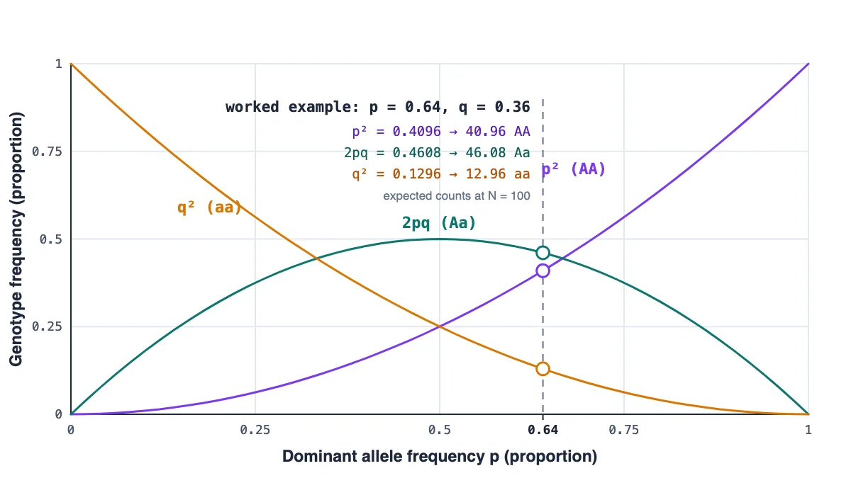
The null model behind p squared plus 2pq plus q squared
Hardy-Weinberg equilibrium is a baseline, not a description of most real populations. If allele frequencies hold from one generation to the next and mating is random, genotype frequencies settle at p squared, 2pq and q squared. The calculator estimates p from your own sample, since each AA contributes two dominant alleles and each Aa one, then multiplies back to expected counts for that sample size.
Two modes cover the two usual situations. Counts mode takes observed AA, Aa and aa tallies and tests them. Frequency mode takes p and a sample size and only prints the expected distribution, which is handy when p comes from a published study rather than your own data. Either way the expected line is the same arithmetic the allele frequency page uses, run in the other direction.
The connection to a Punnett square is worth stating plainly. A grid describes one cross; equilibrium describes a whole gene pool across generations, and the two share the p squared, 2pq and q squared algebra because equilibrium behaves like a population of random one-locus crosses. That is also why the expected line doubles as a carrier-risk engine: the default output predicts 46.08 carriers in a sample of 100, the same arithmetic behind the one-in-N chance a couple is quoted for a recessive condition.
Reading the chi-square result
The test sums each squared deviation from expectation, weighted by the expected value: chi-square equals the sum of (O minus E) squared divided by E. Because p was estimated from the same data, one degree of freedom remains, and the 95th percentile of that distribution sits at 3.84. A statistic above 3.84 means the counts are further from equilibrium than sampling noise comfortably explains; at or below it, the sample is consistent with the model.
The per-genotype breakdown shows where the gap lives. In the default data the heterozygote count sits well below its expectation while both homozygotes run high, which is the classic pattern behind a significant result. The test tells you the pattern, not the cause: inbreeding and subdivided populations both produce it, and so can a batch of genotyping errors.
The per-genotype table is where any diagnosis starts. Each row shows the observed count, the expected count and that genotype's contribution to the total, so the largest term names the class doing the damage. With the defaults, the heterozygote row carries almost all of it: 32 observed against 46.08 expected. Read that pattern alongside the sample size, because a deficit of heterozygotes can come from inbreeding, from pooling structured groups, or from a genotyping assay that misses heterozygous calls, and this test alone cannot tell those stories apart.
Small samples and thin expectations
The chi-square test needs expected counts comfortably above 5. Small samples or extreme allele frequencies push some expectations below that line, and the test then behaves badly, overstating how unusual your counts are. In those cases exact tests are the standard fix, and reporting the observed and expected counts side by side is more honest than a single number.
Sample size also sets the power of the whole exercise. A modest deviation in a sample of fifty will stay under 3.84 even when a real force is acting, because the test cannot see it. Failing to reach the cut-off therefore means only that this sample cannot distinguish the counts from equilibrium, which is a weaker statement than showing the population sits in equilibrium.
For planning, frequency mode does the same arithmetic without a test: enter a published p and a sample size, read off the expected distribution before collecting anything, then decide whether the sample you are about to score can support a chi-square comparison at all.
What the result does not tell you
A significant statistic diagnoses not-equilibrium and stops there. Inbreeding, population subdivision, selection against a genotype, mutation and migration all move counts away from p squared, 2pq and q squared, and several of them produce the same direction of change. Separating them needs more data: family structure, geography, or allele frequencies across multiple loci.
The model itself is narrow. It covers one locus with two alleles, assumes random mating in a large pool with no mutation, migration or selection, and treats genotyping as error-free. Multi-allelic systems such as ABO need a goodness-of-fit per allele instead, and the expected-count rule still applies. Keep those limits next to the number whenever the result feeds a decision.
What your hardy-weinberg equilibrium result means
Hardy-Weinberg is a null hypothesis, not a claim that real populations sit still. Rejecting it tells you some force is present (inbreeding, subdivision, selection, mutation or migration), while failing to reject only means your sample cannot see one.
The expected counts double as a carrier-risk engine: 46.08 expected carriers in this sample is the same arithmetic that says roughly 2pq of a random-mating population carries a recessive condition, the number behind every '1 in N chance' a couple is quoted for a recessive disease.
How to read the output:| Result range | What it means | What to do next |
|---|---|---|
| Above 3.84 | counts too far from p squared, 2pq and q squared | Report a deviation and look for a cause |
| At or below 3.84 | sample consistent with equilibrium | No signal visible at this sample size |
| Expected below 5 | chi-square unreliable | Treat the number as indicative only |
| Largest contribution | the genotype driving the statistic | Start the diagnosis there |
Common mistakes with the hardy-weinberg equilibrium
- Entering p by hand in counts mode: Leave p to be estimated from the counts, otherwise the test compares your input against a derivation of itself.
- Treating a passing test as proof of equilibrium: Passing only means this sample cannot see a force; power stays low when the sample is small or p is extreme.
- Running the test when an expected count is under 5: Exact tests are built for those cases, so report the counts and expectations instead of leaning on chi-square.
- Applying two-allele math to a three-allele system: ABO and similar loci need one goodness-of-fit per allele, because a single p and q cannot describe them.
Limits of the hardy-weinberg equilibrium calculator
The chi-square approximation needs expected counts comfortably above 5. Small samples or extreme allele frequencies push expectations low, and then the test over-rejects: exact tests (like the Wigginton exact test) are the fix for those cases.
p is estimated from the same data, which is why df = 1 rather than 2, and why testing with a literature p you trust is cleaner when you have one. The test is also one-locus and two-allele: multi-allelic systems such as ABO need a per-allele goodness-of-fit instead. Finally, a significant result diagnoses 'not equilibrium' but not which force: Wahlund structure and true inbreeding both show up as heterozygote deficits.
Research note from Dr. Dinesh A. Nagegowda, PhD: Testing population genotype frequencies against the Hardy-Weinberg binomial expansion (p^2 + 2pq + q^2 = 1) requires chi-square goodness-of-fit testing to assess statistical departure from equilibrium. In our ecological genetics fieldwork, departures from equilibrium do not immediately indicate natural selection; small effective population size (genetic drift), non-random assortative mating, or recent migration pulses are equally capable of skewing genotype frequencies.
Sources
- Hardy (1908), Mendelian proportions in a mixed population, Science 28:49-50 (used for: the equilibrium proportions this calculator tests against)
- Hardy (1908) reprint, full text (PubMed Central) (used for: original statement of the random-mating expectation)
- Edwards (2008), G. H. Hardy (1908) and Hardy-Weinberg Equilibrium (used for: interpretation of the equilibrium as a null model rather than a claim about populations)
- Allison (1954), protection afforded by sickle-cell trait, BMJ (used for: example of selection acting on genotype frequencies away from equilibrium)
Cite This Calculator
For laboratory course reports, academic papers, or institutional protocols (APA format):
Hardy-Weinberg Equilibrium: frequently asked questions
What does it mean if the chi-square is significant?
The genotype counts are too far from p², 2pq and q² for sampling noise alone to explain at the 5% level. Candidate causes: inbreeding, population subdivision, selection against a genotype, or genotyping errors. The test flags the problem, not the mechanism.
Why is the critical value 3.84?
It is the 95th percentile of the chi-square distribution with 1 degree of freedom (p was estimated from the data, costing one degree). Any statistic above 3.84 lands in the rejection region at alpha = 0.05.
Can I enter p directly instead of counts?
Yes. Frequency mode computes the expected AA / Aa / aa distribution for any p and sample size without running a test, which is useful for planning or for comparing a sample against a published frequency.
Do I need HWE for a Punnett square?
No. Punnett squares describe a single cross; Hardy-Weinberg describes a whole gene pool across generations. The two share the p² + 2pq + q² algebra because equilibrium is essentially a population of random one-locus crosses.
Found a number that does not match its source? Report a mistake. Corrections are published in place and the page date is updated.
Found a number on this page that doesn’t match its source? Email the correction →.

Dr. Dinesh A. Nagegowda, PhD: Plant & Molecular Biology Editor
Dinesh is a plant molecular biologist and Chief Scientist at CSIR-CIMAP whose research runs through functional genomics, transcriptomics, metabolomics, and biosynthetic pathways in plants. He writes and…