Free Ecology & Environment tool
 Free Ecology & Environment tool
Carrying Capacity Calculator
The Carrying Capacity Calculator calculates population carrying capacity (K) and logistic growth trajectories based on resource limits and intrinsic growth rates (r). Every population grows fast when small, slows as it approaches what the habitat can support, and settles at carrying capacity (K). This calculator runs the logistic equation (the standard model behind wildlife management quotas, fishery yields, and bacteria-in-a-flask curves) and reports where your population sits relative to K at any point in time.
Carrying Capacity Calculator: result
At a glance
- What it does: Runs the logistic equation to project population size and show how much of K is still unused.
- Who it is for: Made for students and wildlife managers estimating harvest quotas or a time-to-target horizon.
- Typical result: Returns population at t, environmental resistance, current surplus and years to a chosen share of K.
How to use the carrying capacity calculator
- Estimate K for your population and habitat: the long-run average the environment supports (carrying capacity from survey data, range assessments, or published site factors). prefill →
- Set N₀ to the current count and r to the intrinsic rate of increase (per year for wildlife, per hour/day for microbes). prefill →
- Pick a time horizon and read the projected population and its share of K.
- Use the target-% field to answer 'how long until the herd reaches 95% of carrying capacity', the question behind harvest quotas.
- Watch environmental resistance: as it approaches 0%, growth stalls no matter how favourable r is.
Carrying Capacity: the formula & its source
Verhulst's logistic equation adds a density-dependent brake to exponential growth. The term (1 − N/K) shrinks as N approaches K:
dN/dt = rN(1 − N/K)
Integrated over time it gives population size at time t:
N(t) = K ÷ (1 + ((K − N₀)/N₀) × e−rt)
And the time to reach any target fraction of K inverts that expression:
t = (1/r) × ln[ N₍target₎(K − N₀) ÷ (N₀(K − N₍target₎)) ]
| Symbol | Meaning | Unit | Typical range |
|---|---|---|---|
K | habitat's long-run sustainable population | individuals | 10 – 1,000,000 |
N₀ | population at the start of the projection | individuals | 1 – K |
r | intrinsic growth rate with resources unlimited | per time unit | 0.01 – 3.0 |
t | time elapsed since the starting count | same unit as r | 0 – 100 |
Target | share of K you want to reach (optional) | % of K | 1 – 99.9 |
Carrying Capacity: worked example
Worked example: a deer herd. K = 500, N₀ = 50, r = 0.2/yr, t = 10 years. N(10) = 500 ÷ (1 + (450/50)e−2) = 500 ÷ (1 + 9 × 0.1353) = 500 ÷ 2.218 = 225 deer (45% of K). Resistance is still 55%, growth is 0.2 × 225 × 0.55 ≈ 24.8 deer/year, and reaching 95% of K takes (1/0.2) × ln[475 × 450 ÷ (50 × 25)] ≈ 25.7 years at this rate.
Example B: target already reached
Example B: already past the target. Count a herd at 480 animals with K = 500 and a 90% target (450 animals), and the time-to-target row reports the level as already reached instead of giving a number. Raise the target to 95% (475 animals) and a positive horizon reappears. The row measures distance from your starting count upward, so it goes quiet only when N₀ already sits above the line you asked about.
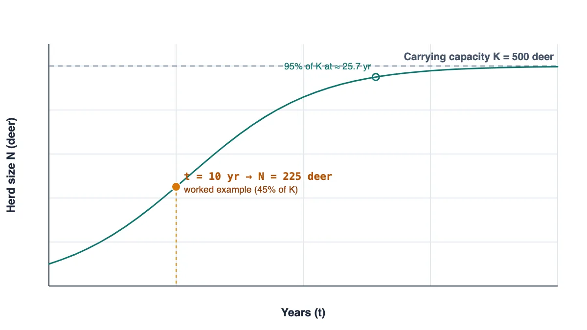
Where the brake comes from
Exponential growth never lasts because resources do not. Verhulst's fix is a single extra term: growth slows in proportion to how much of the habitat's capacity is already taken. With N small, the factor (1 − N/K) sits close to 1 and the population behaves almost exponentially. As N climbs the factor shrinks, and at N = K it hits zero, so growth stops even though r itself never changes.
Three phases follow from that one term. Establishment is slow because few individuals are multiplying. The middle stretch is fast, close to pure exponential growth. Deceleration arrives as resources tighten, and the curve flattens into the familiar S. Environmental resistance is simply the share of K still unused: at 45% of K the resistance is 55%, and per-capita growth is already cut nearly in half compared with an empty habitat.
The calculator reports that brake explicitly alongside the absolute surplus the population is producing right now, so you see both the position on the curve and the pace at that position.
Why the steepest point sits at K/2
Growth rate dN/dt = rN(1 − N/K) is a downward parabola in N, and a parabola peaks halfway between its roots, here at N = K/2. Fishery scientists call that maximum sustainable yield: the population adds the most bodies per unit time there, so a harvest equal to that surplus can repeat every year without shrinking the stock.
Take more than the surplus and the population slides down the far side of the curve, which is how heavily exploited stocks collapse. The practical reading is counter-intuitive. A population at 45% of K looks far from its limit yet may already be near peak production, while one at 90% of K is barely growing. Managers therefore track the count and the surplus derived from it together rather than either number alone, and this calculator puts both rows in front of you.
The same parabola explains why early gains look disappointing. When N is small, even a healthy r multiplies a tiny base, so absolute growth stays modest until the population clears the midpoint. Recovery plans from endangered numbers therefore quote the rate and the count together. A projection sitting well below K/2 after several time units points at r first; one sitting above it warns that the surplus will shrink with every further step toward the limit.
Estimating K you can defend
K is an average, not a wall. It is the long-run population that food, water, shelter and predation can sustain, and it moves with weather, season and habitat change. Take it from survey data, range assessments or published site factors for your area instead of one unusually good year. When two credible sources disagree, run both and report the spread: the difference is honest uncertainty, not an error to hide.
Overshoot belongs in the picture too. Animals reproduce based on past conditions, so a herd can consume past K, damage the resource, and drop below it before the brake responds. Field counts tend to bounce around the ideal curve rather than settle onto it, so treat the projection as the shape of the trend and your survey data as the correction. Age structure also matters: a herd of mostly juveniles will grow for a while faster than the same count of adults, a detail this single-rate model averages away.
How to read the time-to-target row
The target field answers the question behind most harvest quotas: how long until this herd reaches 95% of K. Because the answer comes from inverting the logistic curve, every input pushes it around. A small r stretches the horizon sharply, a start far below the target stretches it further, and a target very close to 100% stretches it without end. The last sliver of K arrives extremely slowly.
Match units and the row reports in them: r per year gives a horizon in years. When the row says the level is already reached, your starting count sits above the target, so either raise the target or accept that the question does not apply here. Treat every figure as a first-order projection, validate it against survey counts before the number drives a quota, and revisit K whenever habitat conditions change.
A useful cross-check sits in the projection itself: step forward one time unit and compare the predicted count with your next survey. Misses repeating in the same direction mean K or r is wrong rather than the wildlife. Refreshing either input from fresh data is normal practice: the model earns its keep by being rerun against reality, not by being right the first time.
What your carrying capacity result means
The curve's signature is the S-shape: slow establishment, exponential middle, deceleration as resistance builds. Maximum sustainable yield in fisheries and harvest quotas in wildlife management target the steepest part of the curve (N = K/2), where dN/dt peaks. Take more than that surplus and the population slides down the curve.
Environmental resistance is the fraction of the habitat's capacity not yet consumed: at 45% of K, competition, predation, and resource limitation are already cutting the growth rate nearly in half relative to its peak.
How to read the output:| Result range | What it means | What to do next |
|---|---|---|
| under 50% of K | exponential middle, surplus climbing | Good window for measuring r in the field |
| near 50% of K | steepest point of the curve | Surplus peaks here: the quota reference point |
| above 90% of K | resistance nearly total | Expect slow gains; overshoot risk if r stays high |
| target time grows sharply | small r, far start, or target near 100% | Check units and inputs before quoting the horizon |
Common mistakes with the carrying capacity
- Feeding r per year against t in generations: Set both on one clock: if t counts years, r must be per year. The field hint spells out the unit the rate is quoted in.
- Treating K as a constant written in stone: K drifts with weather, season and habitat change. Refresh it from recent surveys and rerun the projection each planning cycle.
- Reading a big count as a fast-growing population: Growth peaks at K/2, so a population near K is barely increasing. Check the current surplus row before assuming momentum.
- Quoting time-to-target without validating it: The formula assumes a fixed K and instant feedback. Confirm the horizon against observed counts before it sets a harvest quota.
Limits of the carrying capacity calculator
The logistic model assumes one limiting resource, instant density feedback, a fixed K, and no age structure, none of which hold exactly in the field. Real K moves with weather, season, and habitat change, and populations routinely overshoot it. Treat outputs as a first-order projection, then validate against survey data before setting a quota.
Fieldwork note from Dr. Dinesh A. Nagegowda, PhD: In population ecology, modeling carrying capacity (K) using the logistic growth equation assumes resource availability remains constant over time. In real-world ecosystems, K is a dynamic, moving target that fluctuates with seasonal rainfall, vegetative productivity, and predator pressure. When animal populations overshoot carrying capacity due to delayed density-dependent feedback, they degrade the resource base, causing subsequent population crashes below original baseline levels.
Sources
- Begon, Townsend & Harper, Ecology: Individuals, Populations and Communities (WorldCat record) (used for: logistic model treatment and the definition of carrying capacity)
- OpenStax Biology 2e: Environmental Limits to Population Growth (used for: density dependence, environmental resistance and K in plain language)
- OpenStax Biology 2e: Population Dynamics and Regulation (used for: overshoot, regulation and the factors that move K)
Cite This Calculator
For laboratory course reports, academic papers, or institutional protocols (APA format):
Carrying Capacity: frequently asked questions
What is carrying capacity (K)?
The average population size the environment can sustain indefinitely given food, water, shelter, and predation: the level dN/dt settles at.
What does r mean in the logistic equation?
The intrinsic rate of increase: per-capita growth when resources are unlimited. r = 0.2 means the population would grow 20% per time unit in the absence of density effects.
Why does growth peak at K/2?
dN/dt = rN(1 − N/K) is a downward parabola in N, maximized at N = K/2, the basis of maximum sustainable yield in fisheries and harvest management.
Why do real populations overshoot K?
Feedback lags: animals reproduce based on past conditions, so they can consume past K, degrade the resource, and crash below it before the brake takes effect.
Found a number that does not match its source? Report a mistake. Corrections are published in place and the page date is updated.
Something on this page not matching its cited source? Report it.

Dr. Dinesh A. Nagegowda, PhD: Plant & Molecular Biology Editor
Dinesh is a plant molecular biologist and Chief Scientist at CSIR-CIMAP whose research runs through functional genomics, transcriptomics, metabolomics, and biosynthetic pathways in plants. He writes and…